The Electronic Computers, Part 3: ENIAC

The second electronic computing project to emerge from the war, like Colossus, required many minds (and hands) to bring it to fruition. But, also like Colossus, it would have never come about but for one man’s fascination with electronics. In this case, the man’s name was John Mauchly.

Mauchly’s story intertwines in curious (and, to some, suspicious) ways with that of John Atanasoff. As you will recall,  we last left Atanasoff and his assistant, Claude Berry, in 1942. Having abandoned their own electronic computer to take on other work for the war. Mauchly had quite a bit in common with Atanasoff: both were physics professors at  lesser-known institutions, with no prestige or authority in the wider academic community. Mauchly languished in particular obscurity, as a teacher at little Ursinus College outside Philadelphia, which lacked even the modest prestige of Atanasoff’s Iowa State. Neither had done anything to merit the notice of their elite brethren at, say, the University of Chicago. Yet both were taken with the same eccentric idea: to build a computing machine from electronic components, the same parts used to make radios or telephone amplifiers.

Predicting the Weather

For a time, these two like-minded men formed a bond, of sorts. They met in late 1940, at a conference of the American Association for the Advancement Science (AAAS) in Philadelphia. There, Mauchly presented a paper on his study of cyclical patterns in weather data, using an electronic harmonic analyzer he had designed. It was an analog computer¹ similar in function to the mechanical tide predictor devised by William Thomson (later Lord Kelvin) in the 1870s.

Atanasoff, sitting in the audience, knew he had found a fellow-traveler on the lonely road to electronic computing, and he did not hesitate to approach Mauchly after the talk to tell him about the machine he was building in Ames. But to understand how Mauchly ended up presenting a paper on an electronic weather computer in the first place, we must go back to his roots.

Mauchly was born in 1907 as the son of another physicist, Sebastian Mauchly. Like many of his contemporaries, he developed an interest as a boy in radios and vacuum-tubes, and he vacillated between electrical engineering and physics before deciding to focus on meteorology at Johns Hopkins. Unfortunately, he graduated from his Ph.D. program into the teeth of the Great Depression, and felt lucky to land a position at Ursinus in 1934, as the solitary member of its physics department.

At Ursinus, he began his dream project – to unveil the hidden cycles of the global weather machine, and thus learn to predict the weather not days, but months or years in advance. He was convinced that the sun drove multi-year weather patterns related to levels of sunspot activity. He would extract these patterns of solar gold from the vast silt of data at the U.S. Weather Bureau, with the help of a team of students and a bank of desk calculators acquired at a cut rate from collapsed banks.

It soon became apparent, though, that there was simply too much data – too much silt to pan through. The machines could not compute fast enough, and moreover human error was introduced by the constant need to copy intermediate results from machine to paper. Mauchly began to think about another way. He knew about the vacuum tube counters pioneered by Charles Wynn-Willliams that his fellow physicists used to count sub-atomic particles. Given that electronic devices could clearly record and accumulate numbers, Mauchly wondered, why could they not perform more complex calculations? He spent several years of his spare time fiddling with electronic components: flip-flops, counters, a substitution cipher machine that used a mix of electronic and mechanical parts, and finally the harmonic analyzer, which he applied to his weather-prediction project, extracting what looked like multi-week patterns of rainfall variation in the U.S weather data. This is the finding that brought Mauchly to the AAAS in 1940, and the finding that brought Atanasoff to Mauchly.

The Visit

The pivotal event of Mauchly and Atanasoff’s relationship came about six months later, early in the summer of 1941. In Philadelphia, Atanasoff had told Mauchly about the electronic computer he was building in Iowa, and mentioned how cheaply he had managed to build it. In their correspondence afterward, he continued to make teasing hints about how he had built his computer at less than $2 per digit in hardware cost. Mauchly was intrigued, amazed even, by this achievement. By this time, he was entertaining serious plans for building an electronic calculator, but with no support from his college, he would have to pay for all the equipment out of his own pocket. A single tube typically cost $4, and it would take two tubes to store even a single binary digit in a typical flip-flop circuit. How, he wondered, could Atanasoff have possibly achieved such economy?

Six months later, he was finally able to find the time to head west to satisfy his curiosity.  After a thousand mile cross-country drive, Mauchly and his son arrived at Atanasoff’s home in Ames in June 1941. Mauchly would later say that he came away disappointed. Atanasoff’s inexpensive storage was not electronic at all, but held in electro-static charges on a mechanical drum. Because of this and other mechanical parts, as we saw earlier, it could not compute at nearly the speed Mauchly dreamed of. He later called it “a mechanical gadget that uses some electronic tubes.”² Yet shortly after the visit he wrote a letter praising Atanasoff’s machine, writing that it was “electronic in operation, and will solve within a very few minutes any system of linear equations involving no more than thirty variables.”  He claimed it would be both faster and cheaper than the mechanical Bush differential analyzer.³

Some three decades on, Mauchly and Atanasoff’s relationship would become pivotal to the arguments in Honeywell v. Sperry Rand, the court case whose ultimate resolution invalidated Mauchly’s patent claims to an electronic computer. Without commenting on the inherent merits of the patent itself, and allowing for the fact that Atanasoff was surely the more accomplished engineer, and granting that Mauchly’s retrospective opinions of Atanasoff and his computer are deeply suspect, still there is no reason to believe that Mauchly learned or copied anything of significance from Atanasoff. Clearly Mauchly’s general idea for an electronic computer did not come from Atanasoff. But more importantly, in no point of detail does the design of the later ENIAC have anything in common with the Atanasoff-Berry Computer. At most one could say that Atanasoff bolstered Mauchly’s confidence, providing an existence proof that electronic computing could work.

The Moore School and Aberdeen

Meanwhile, Mauchly was left where he had started. There was no magic trick for cheap electronic storage, and as long as he remained at Ursinus, he lacked the means to make his electronic dream a reality. Then came his lucky break. That same summer of 1941, he attended a summer course on electronics at the University of Pennsylvania’s Moore School of Engineering. By this time France was subjugated and Britain under siege, U-boats prowled the Atlantic, and American relations with an aggressive, expansionist Japan were deteriorating rapidly. Despite the isolationist bent of the populace as a whole, American intervention seemed probable, if not inevitable, to the elite at places like the University of Pennsylvania. The Moore School thus offered a course to bring scientists and engineers up to speed in preparation for possible wartime work, especially on the topic of radar technology.⁴

This course had two crucial consequences for Mauchly: first, it brought him in contact with Presper (Pres) Eckert, scion of a local real-estate empire and a young electronics whiz who had whiled away his teenage afternoons in the lab of television pioneer Philo Farnsworth. Eckert would later share authorship of the (ultimately invalidated) ENIAC patent with Mauchly. Second, it landed him a position in the Moore School faculty, ending his long academic isolation at the backwater of Ursinus College. This, it seems, was not due to any special merit on Mauchly’s part, but simply because the school was desperate for bodies to replace the academics that were being pulled into full-time war work.

By 1942, however, a large part of the Moore School itself was taken over by a war project of its own: the computing of ballistic firing trajectories by mechanical and manual means. This project grew organically out of the school’s pre-existing relationship with the Aberdeen Proving Ground, about eighty miles down the coast in Maryland.

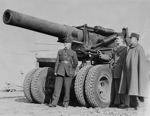
The Proving Ground was created during the First World War to provide gunnery testing services to the Army, replacing the previous testing ground at Sandy Hook, New Jersey. In addition to actually test-firing weapons, it had the task of computing firing tables for use by artillery units in the field. Due to the complicating factor of air resistance, it was not possible to determine where a shell would land when fired from a gun by simply solving a quadratic equation. Nonetheless, high precision and accuracy were extremely important to artillery fire given that the initial shells were the most likely to kill and maim – after that the targeted men would go to ground as quickly as possible.

To achieve such precision, modern armies built extensive tables which told gunners precisely how far away their shell would land when fired at a given angle. The tabulators used the shell’s initial velocity and position to compute the position and velocity a short time interval later, and then repeated the same computation for the next time step, and so on for hundreds or thousands of repetitions. For each combination of gun and shell, the same computations had to be made for every possible angle of fire, and accounting for a variety of different atmospheric conditions. The load of calculation was so massive that it took Aberdeen until 1936 to finish out the firing tables that it began at the conclusion of the First World War.

Obviously, Aberdeen was in the market for a better solution. In 1933, it made a deal with the Moore School: the Army would provide the money to build two differential analyzers, analog computers modeled on the MIT design overseen by Vannevar Bush. One would be shipped down to Aberdeen, but the other would remain on loan at the Moore School for whatever use its professors saw fit. The analyzer could plot a trajectory in fifteen minutes that would have taken a human computer multiple days, albeit with somewhat less precision.

In 1940, however, the research division, now called the Ballistic Research Laboratory (BRL), called in its loan, and took over the Moore School machine to begin plotting artillery tables for the looming war. The school’s computing group was also pulled in to supplement the machine with human calculation. By 1942, 100 woman computers at the school were working six days a week to churn out computations for the war – among them was Mauchly’s wife, Mary, who worked on Aberdeen’s firing tables. Mauchly himself was put in charge of another group of computers working on radar antenna calculations.

Ever since arriving at the Moore School, Mauchly had been shopping his idea for an electronic computer around among the faculty. Already he had some significant allies, including Presper Eckert and John Brainerd, a more senior faculty member. Mauchly provided the vision, Eckert the engineering chops, and Brainerd the credibility and legitimacy. In the spring of 1943, the three decided the time was right to pitch Mauchly’s long-simmering idea directly to the Army. But the mysteries of the climate that he had long hoped to unveil would have to wait. His new computer would serve the needs of a new master: tracing not the eternal sinusoids of global temperature cycles, but the all-too-mortal ballistic arcs of artillery shells.

ENIAC

In April 1943, Mauchly, Eckert, and Brainerd drafted a “Report on an Electronic Diff. Analyzer.” It quickly acquired them another ally, Herman Goldstine, a mathematician and Army officer who served as the liaison between Aberdeen and the Moore School. With Goldstine’s help, the group pitched their idea to a committee at the BRL, and got an Army grant to fund their project, with Brainerd as the principal investigator. They were to finish the machine by September 1944, with a budget of $150,000. The team dubbed their project ENIAC: Electronic Numerical Integrator, Analyzer and Computer.

As with Colossus in the U.K., the established engineering authorities in the U.S., such as the National Defense Research Committee (NDRC), received the ENIAC proposal with skepticism. The Moore School did not have the reputation of an elite institution, yet it proposed to build something unheard of. Even industrial giants like RCA had struggled to build relatively simple electronic counting circuits, much less a highly configurable electronic computer.⁵ George Stibitz, architect of the Bell relay computers and now part of the NDRC computing projects committee, believed that ENIAC would take far too long to build to be useful to the war.

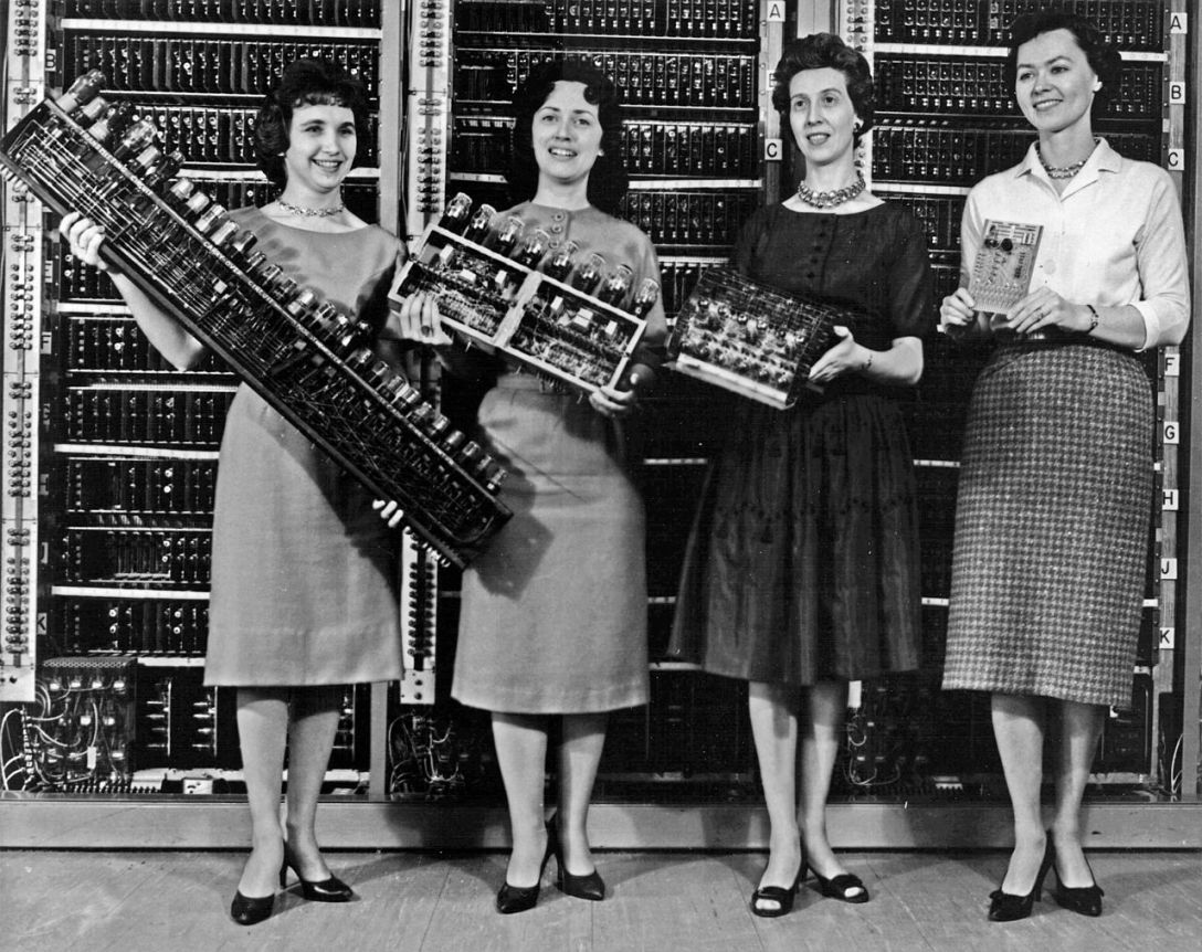
In that he proved correct. ENIAC would take more than twice as long and cost three times as much as originally planned. It sucked up a huge portion of the human resources of the Moore School. The design work alone required the help of seven others in addition to the initial group of Mauchly, Eckert, and Brainerd. As with Colossus, the ENIAC project co-opted many of the school’s human computers to help configure their electronic replacement, among them Herman Goldstine’s wife Adele, and Jean Jennings (later Bartik), both of whom later did important work of their own in computer design. As the “NI” in ENIAC suggests, the Moore School team sold the Army on a digital, electronic, version of the differential analyzer, which would solve integrations for trajectories far faster and more precisely than its analog, mechanical counterpart.⁶ But what they delivered was rather more than that.

The core of the ENIAC’s capabilities, again as with Colossus, came from its variety of functional units. The most used were accumulators for adding and counting. Their design derived directly from the Wynn-Williams-style electronic counters used by physicists, and they literally added by counting, in the way that a preschooler might add on his fingers. Other functional units included multipliers and function generators for doing table look-ups to shortcut more complex functions (such as sine and cosine). Each functional unit had local program controls to set up short sequences of operations. As with Colossus, programming was done with a combination of panel switches and telephone-style plugboards.

ENAIC also had some electro-mechanical parts, notably the relay register that served as a buffer between the electronic accumulators and the IBM punch card machines used for input and output. Again this was much the same architecture as Colossus. Sam Williams of Bell Labs, who had collaborated with George Stibitz on the construction of the Bell relay computers, also built the register for ENIAC.

But one key difference from Colossus made ENIAC a far more flexible machine: its programmable central control. The master programmer unit sent pulses to the functional units to trigger a pre-programmed sequence, and received a return pulse when the unit finished. It then went on to the next operation in its master coordination sequence, producing the overall desired computation as a function of many of these small sequences. The master programmer could also make decisions, or branches, by using a stepper: a ring counter that determined to which of six output lines an input pulse would be forwarded. Thus the master could execute up to six different functional sequences depending on the current state of the stepper. This flexibility would enable ENIAC to solve problems far removed from its initial bailiwick of ballistic computations.

Eckert was responsible for keeping all the electronics in this monstrosity humming, and independently came up with the same basic tricks as Flowers at Bletchley: run the filaments at well below their rated current, and never turn the machine off. Because of the huge number of tubes involved, however, another trick was required: plug-in units holding several dozen tubes that could be quickly swapped out in case of failure. Maintenance workers would then find and replace the precise failed tube at leisure while ENIAC returned to work immediately. Even with all these measures, given the vast number of tubes in ENIAC, it could not crank away on a problem over the weekend or even overnight, as relay computers routinely did. Invariably a tube would fail.

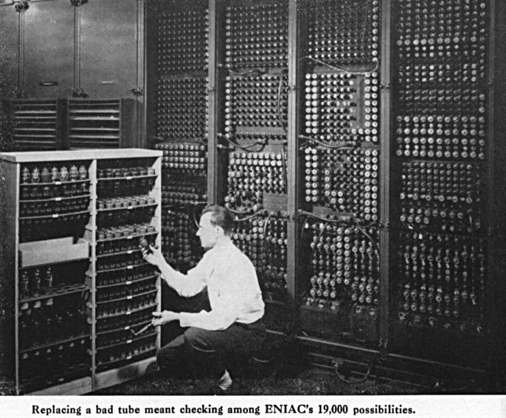
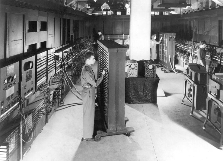
Accounts of the ENIAC  often emphasize its tremendous size. Its many racks of tubes – 18,000 of them in total – switches, and plugboards would fill a typical ranch house and overflow into the front yard. Its size was a product not merely of its components (tubes were relatively large) but of its peculiar architecture. Though all mid-century computing machines appear gigantic by modern standards, the next iteration of electronic computers were far smaller than ENIAC, providing greater capability with one-tenth the number of electronic components.

ENIAC’s grotesque size proceeded directly from two major design choices. The first traded off cost and complexity for potential speed. Virtually all later computers instead stored numbers in registers and then processed them through a separate arithmetic unit, storing the result back into a register. ENIAC, however, had no separation between storage and processing units: each number storage location was also a processing unit that could add and subtract, and thus required many extra tubes. It could be seen as simply a massively accelerated version of the Moore School’s human computing division, for it “had the computational architecture of a roomful of twenty computers working with ten-place desk calculators and passing results back and forth.”⁷ In theory this allowed ENIAC to compute in parallel across multiple accumulators, but that capability was little used, and was removed in 1948.

The second design choice is harder to defend on any grounds. Unlike the ABC or the Bell relay machines, ENIAC did not store numbers in a binary representation. Instead it translated a decimal mechanical counting wheel directly into electronics, with ten flip-flops per digit – if the first was lit up, that was a 0, the second a 1, the third a 2, etc. This was hugely wasteful of expensive electronic components,⁸ and seems to have been done solely out of fear of the complexity of binary-decimal conversion during input and output. Yet the Atanasoff-Berry Computer, Colossus, and the Bell and Zuse relay machines all used binary internally and their designers had no great difficulty with converting between bases.

These design choices would not be repeated. In this sense, ENIAC was like the ABC – a one-off oddity rather than the template for all modern computing machines. However it was different in one very important sense – it proved beyond a shadow of a doubt the viability of electronic computing, by doing useful work, solving real problems with incredible speed, in the public eye.

Vindication

By November 1945, ENIAC was fully functioning. It could not boast the same robustness as its electromechanical cousins, but it was reliable enough for its several-hundred-fold speed advantage to tell. Whereas the differential analyzer took fifteen minutes, ENIAC could compute a ballistic trajectory in twenty seconds – less than the actual flying time of the shell.⁹ And, unlike the analyzer, it did so with the same precision as a human computer using a mechanical calculator.

As Stibitz had predicted, however, ENIAC arrived too late to contribute to the war effort, and there was no longer a pressing need for artillery tables. But there was a secret weapons project operated out of Los Alamos, New Mexico that had acquired a momentum of its own, and continued to operate after the war. It also continued to hunger for calculation. One of the Manhattan Project physicists, Edward Teller, had become taken as early as 1942 with the idea of a “Super”: a far more powerful weapon than those later dropped on Japan, whose explosive energy would come from atomic fusion, rather than fission. Teller believed he could ignite a fusion chain reaction in a mixture of deuterium (normal hydrogen plus one neutron) and tritium (normal hydrogen plus two neutrons). But for that to be feasible, the proportion of tritium required had to be low, for it was extremely rare.

The Los Alamos scientists therefore brought to the Moore School a calculation to test the feasibility of the Super, by computing differential equations that modeled the ignition of a deuterium-tritium mix at various concentrations of tritium. No one at the Moore School had the clearance to know what the calculation was actually for, but they dutifully set up the data and equations provided by the Los Alamos scientists. In fact, the details of the calculation remain classified to this day (as does the entire program to build the “Super,” now known more commonly as the hydrogen bomb), though we know that Teller considered the result, rendered in February 1946, a vindication of his design.¹⁰

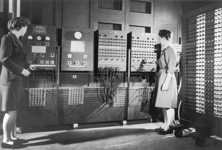
That same month, the Moore School gave ENIAC its public debut. In a ritual unveiling before assembled VIPs and the press, operators pretended to turn on the machine (though of course it was always on), then ran it through some ceremonial calculations, computing a ballistic trajectory to show off the unprecedented speed of its electronic components. Afterward, the staff distributed punched card outputs from the calculation to each attendee.

ENIAC went on to solve several more real problems during the remainder of 1946: a series of calculations on the flow of fluids (such as airflow over a wing) by British physicist Douglas Hartree, another Los Alamos calculation for modeling the implosion of a fission weapon, some trajectory calculations for a new ninety-millimeter cannon for Aberdeen. Then it fell silent for a year and a half. At the end of 1946, as part of the Moore School’s agreement with the Army, BRL packed up the machine and moved it down to the proving ground. Once there it suffered from persistent reliability problems, and the BRL team did not get it working smoothly enough to do any useful work until after a major overhaul, completed in March 1948.¹¹

It didn’t matter. No one was paying attention to ENIAC any more. The race was already on to build its successor.

Further Reading

Paul Ceruzzi, Reckoners (1983)

Thomas Haigh, et. al., Eniac in Action (2016)

David Ritchie, The Computer Pioneers (1986)